Customize grid, colors, and tick labels
This notebook focuses on presentation controls for Smith charts:
turning major/minor grids on and off
changing the number of major divisions (tick locations)
changing minor grid density
enabling the “fancy” grid style
controlling tick-label formatting (precision, symmetry)
changing grid colors (major/minor separately)
Recommended configuration pattern
pysmithchart supports both:
smith_params={...}(recommended for clarity), anddirect dot-notation kwargs like
**{'grid.Z.major.enable': True}(backwards compatible).
In documentation, a practical pattern is to define a reusable configuration dictionary and pass it with **config:
sc = {
    "grid.Z.major.enable": True,
    "grid.Z.minor.enable": False,
}
ax = plt.subplot(111, projection="smith", **sc)
[1]:
%config InlineBackend.figure_format = 'retina'

import sys
import numpy as np
import matplotlib.pyplot as plt

if sys.platform == "emscripten":
    import piplite

    await piplite.install("pysmithchart")

import pysmithchart
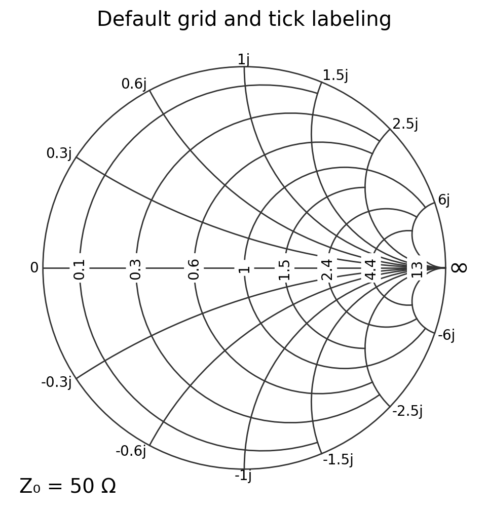
1. Default grid and ticks
[2]:
sc = {}
plt.figure(figsize=(6, 6))
ax = plt.subplot(111, projection="smith", **sc)
ax.set_title("Default grid and tick labeling")
plt.show()
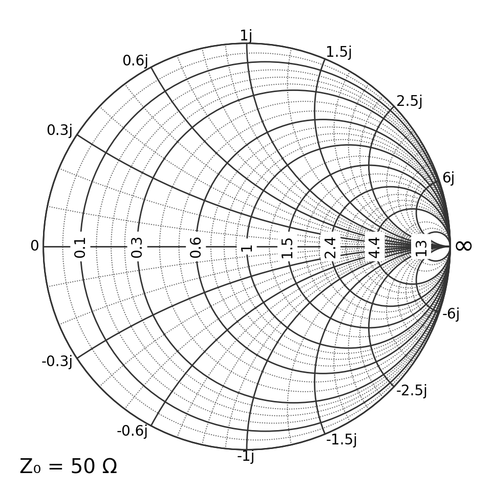
2. Enable/disable major and minor grids (reusable config)
This uses dot-notation keys passed directly as kwargs.
[3]:
sc = {
    "grid.Z.major.enable": True,
    "grid.Z.minor.enable": True,
    "grid.Z.minor.real.divisions": None,
    "grid.Z.minor.imag.divisions": None,
    "grid.fancy": False,
}

plt.figure(figsize=(6, 6))
ax = plt.subplot(111, projection="smith", **sc)
plt.show()
Updating an existing axes
If the axes already exists, update the Smith-chart parameters and then rebuild the chart:
ax.update_scParams(**{"grid.Z.minor.enable": True})
ax.clear()
clear() is important because gridlines/tick locators are assembled during Smith-chart initialization.
[14]:
sc = {"grid.Z.minor.enable": False}
plt.figure(figsize=(6, 6))
ax = plt.subplot(111, projection="smith", **sc)
ax.set_title("Minor grid toggled ON after creation")

ax.update_scParams(**{"grid.Z.minor.enable": True})
ax.clear()  # rebuild to apply locator/grid settings
plt.show()
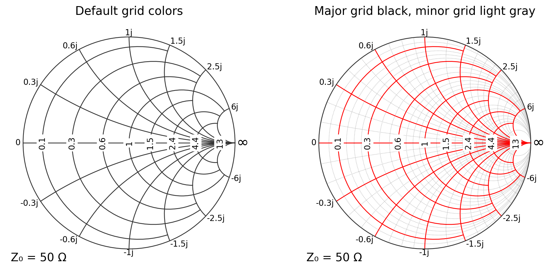
3. Changing grid colors
You can change major/minor grid colors independently:
grid.Z.major.colorgrid.Z.minor.color
This is particularly useful for classroom figures where you want the major grid to stand out.
[5]:
plt.figure(figsize=(12, 6))

# Default colors
ax1 = plt.subplot(121, projection="smith")
ax1.set_title("Default grid colors")

# Customized colors
sc_color = {
    "grid.Z.major.enable": True,
    "grid.Z.minor.enable": True,
    "grid.Z.major.color": "red",
    "grid.Z.minor.color": "0.7",  # grayscale string is convenient
}
ax2 = plt.subplot(122, projection="smith", **sc_color)
ax2.set_title("Major grid black, minor grid light gray")

plt.show()
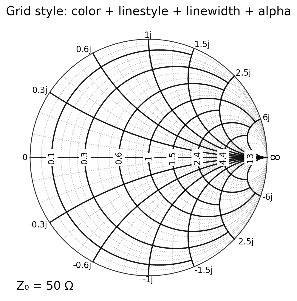
Color + line styling together
Common style keys include:
grid.Z.major.linestyle,grid.Z.major.linewidth,grid.Z.major.alphagrid.Z.minor.linestyle,grid.Z.minor.linewidth,grid.Z.minor.alpha
[6]:
sc_style = {
    "grid.Z.major.enable": True,
    "grid.Z.minor.enable": True,
    "grid.Z.major.color": "black",
    "grid.Z.major.linestyle": "-",
    "grid.Z.major.linewidth": 1.5,
    "grid.Z.major.alpha": 0.9,
    "grid.Z.minor.color": "0.7",
    "grid.Z.minor.linestyle": "--",
    "grid.Z.minor.linewidth": 1.0,
    "grid.Z.minor.alpha": 0.8,
}

plt.figure(figsize=(6, 6))
ax = plt.subplot(111, projection="smith", **sc_style)
ax.set_title("Grid style: color + linestyle + linewidth + alpha")
plt.show()
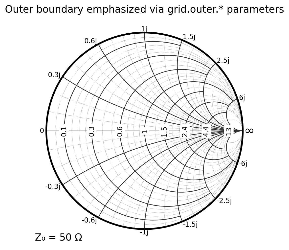
3a. Styling the outer boundary (Smith-circle frame)
The outer Smith-chart boundary (the chart frame) is now controlled through Smith-chart parameters:
grid.outer.enablegrid.outer.colorgrid.outer.linestylegrid.outer.linewidthgrid.outer.alpha
This is useful when you want the boundary to stand out more strongly than the grid, especially in teaching figures.
[7]:
# Boundary styling example
sc_boundary = {
    "grid.Z.major.enable": True,
    "grid.Z.minor.enable": True,
    "grid.Z.major.color": "0.2",
    "grid.Z.minor.color": "0.7",
    "grid.outer.enable": True,
    "grid.outer.color": "black",
    "grid.outer.linewidth": 2.5,
    "grid.outer.linestyle": "-",
    "grid.outer.alpha": 1.0,
}

plt.figure(figsize=(6, 6))
ax = plt.subplot(111, projection="smith", **sc_boundary)
ax.set_title("Outer boundary emphasized via grid.outer.* parameters")
plt.show()
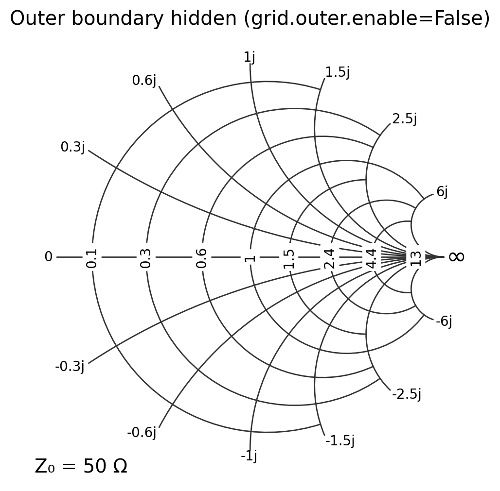
[8]:
# Hiding the outer boundary entirely (occasionally useful for overlays)
sc_no_boundary = {
    "grid.outer.enable": False,
}

plt.figure(figsize=(6, 6))
ax = plt.subplot(111, projection="smith", **sc_no_boundary)
ax.set_title("Outer boundary hidden (grid.outer.enable=False)")
plt.show()
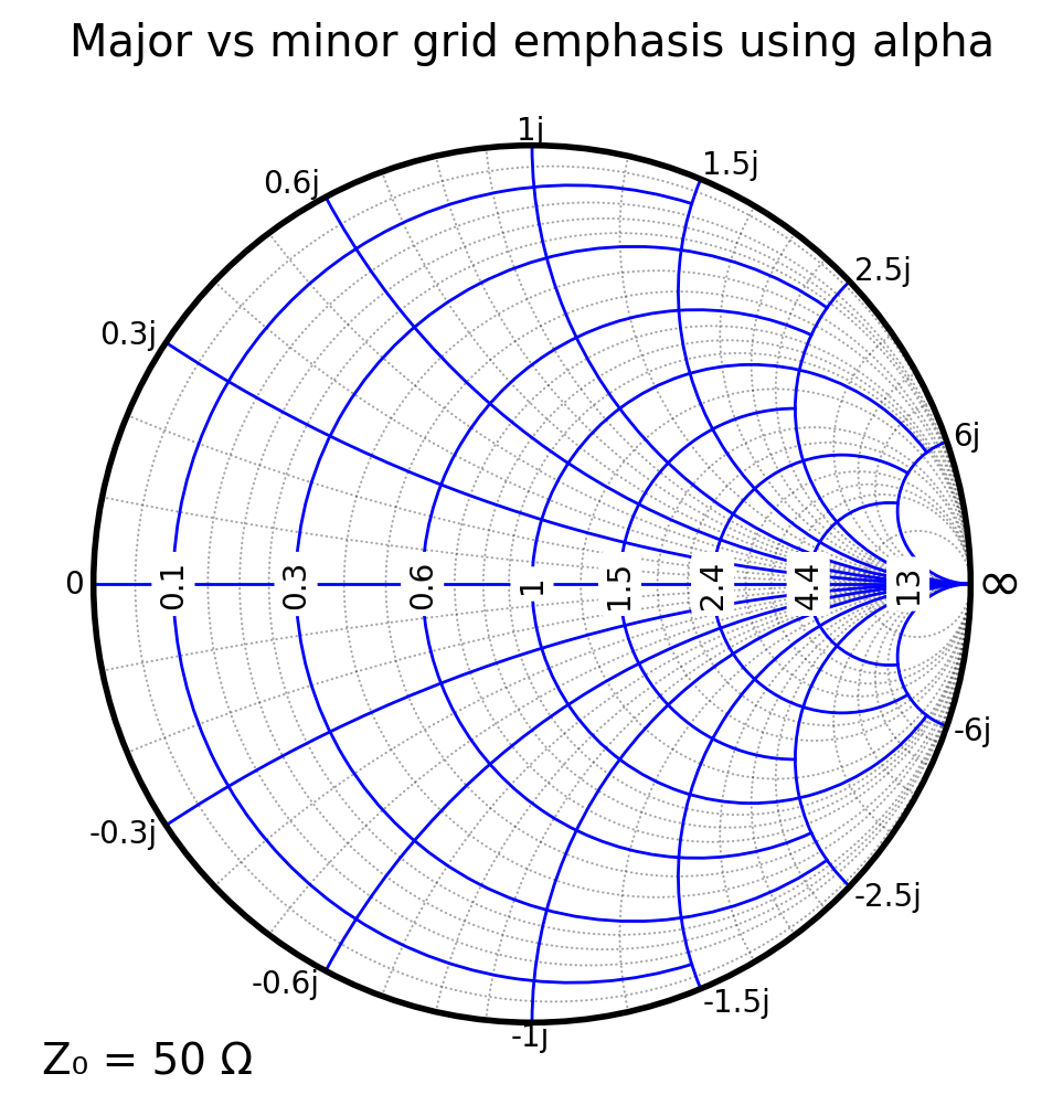
3b. Using alpha to emphasize major vs minor grids
With grid.Z.major.alpha and grid.Z.minor.alpha, you can keep grid colors the same but visually emphasize the major grid using transparency.
This is especially effective for lecture figures and slides, where you want students to focus on the major resistance/reactance circles without losing the minor-grid context.
[16]:
# Same colors, different alpha values
sc_alpha = {
    "grid.Z.major.enable": True,
    "grid.Z.minor.enable": True,
    "grid.Z.major.color": "blue",
    "grid.Z.minor.color": "black",
    "grid.Z.major.alpha": 1.0,  # fully opaque
    "grid.Z.minor.alpha": 0.35,  # lighter minor grid
    "grid.outer.color": "black",
    "grid.outer.linewidth": 2.0,
}

plt.figure(figsize=(6, 6))
ax = plt.subplot(111, projection="smith", **sc_alpha)
ax.set_title("Major vs minor grid emphasis using alpha")
plt.show()
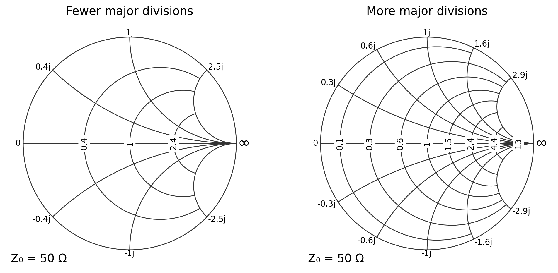
4. Changing the number of major divisions (tick locations)
Major tick placement is controlled by:
grid.Z.major.xmaxn(real-axis divisions / resistance circles)grid.Z.major.ymaxn(imag-axis divisions / reactance arcs)
[10]:
plt.figure(figsize=(12, 6))

sc = {"grid.Z.major.real.divisions": 4, "grid.Z.major.imag.divisions": 6}
ax = plt.subplot(121, projection="smith", **sc)
ax.set_title("Fewer major divisions")

sc = {"grid.Z.major.real.divisions": 10, "grid.Z.major.imag.divisions": 12}
ax = plt.subplot(122, projection="smith", **sc)
ax.set_title("More major divisions")

plt.show()
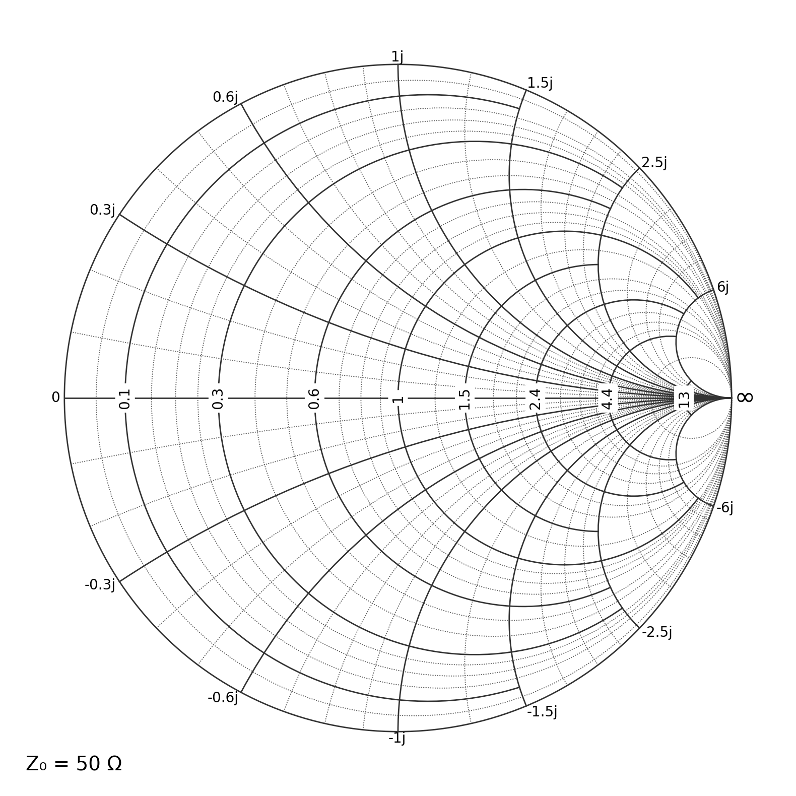
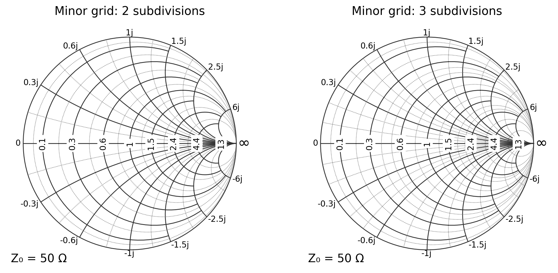
5. Minor grid density
Minor tick placement is controlled by:
grid.Z.minor.xauto(minor subdivisions between major x ticks)grid.Z.minor.yauto(minor subdivisions between major y ticks)
[15]:
sc1 = {
    "grid.Z.minor.enable": True,
    "grid.Z.minor.real.divisions": 2,
    "grid.Z.minor.imag.divisions": 2,
}

sc2 = {
    "grid.Z.minor.enable": True,
    "grid.Z.minor.real.divisions": 3,
    "grid.Z.minor.imag.divisions": 3,
}

plt.figure(figsize=(12, 6))

ax1 = plt.subplot(121, projection="smith", **sc1)
ax1.set_title("Minor grid: 2 subdivisions")

ax2 = plt.subplot(122, projection="smith", **sc2)
ax2.set_title("Minor grid: 3 subdivisions")

plt.show()
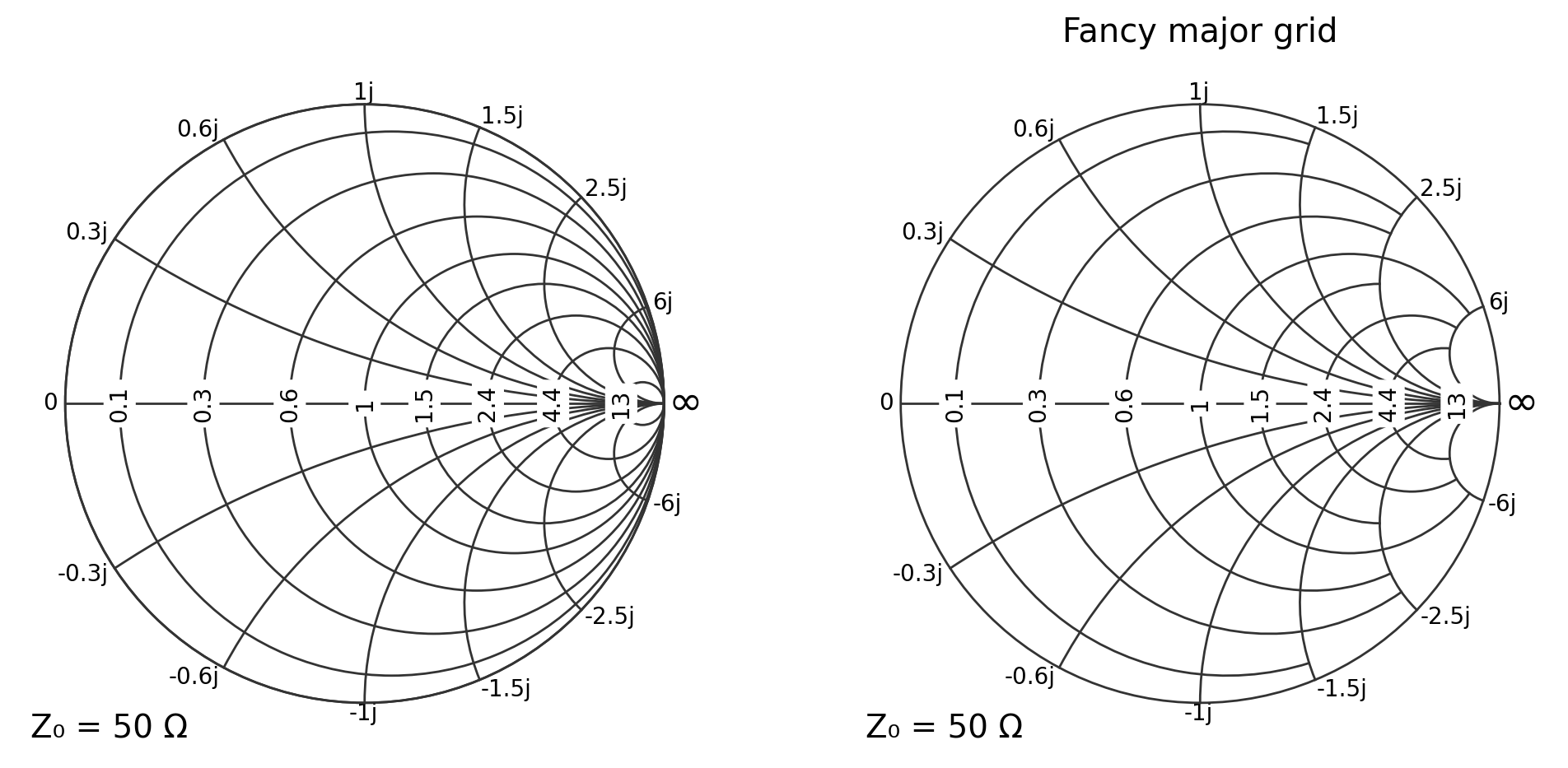
6. “Fancy” grid style
pysmithchart supports a “fancy” grid mode that adaptively shortens grid segments to avoid clutter. To draw a fancy grid, call:
ax.grid(True, which="major", axis=True)
This is most useful for major gridlines.
[12]:
sc1 = {"grid.fancy": False}
sc2 = {"grid.fancy": True}
plt.figure(figsize=(12, 6))

# Standard major grid
ax = plt.subplot(121, projection="smith", **sc1)
ax1.set_title("Standard major grid")

# Fancy major grid
ax2 = plt.subplot(122, projection="smith", **sc2)
ax2.set_title("Fancy major grid")

plt.show()
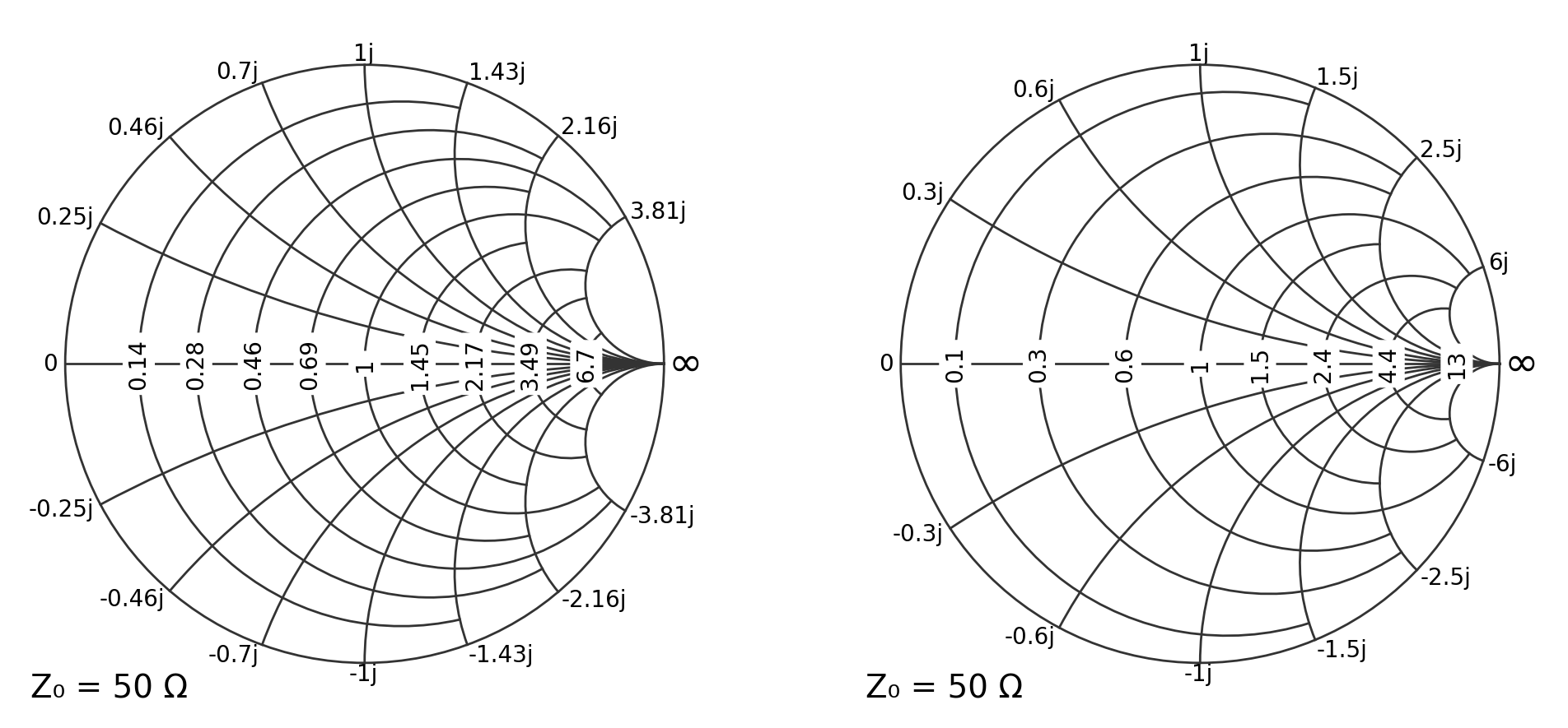
7. Tick-label formatting and precision
A practical control is the rounding precision used by the major tick locators:
grid.locator.precision
[13]:
sc1 = {"grid.locator.precision": 4}
sc2 = {"grid.locator.precision": 2}
plt.figure(figsize=(12, 6))

ax = plt.subplot(121, projection="smith", **sc1)
ax1.set_title("Locator precision = 2")

ax = plt.subplot(122, projection="smith", **sc2)
ax2.set_title("Locator precision = 4")

plt.show()
Summary
For reusable configuration, build a dict of dot-notation keys and pass it with
**config.Common knobs:
enable:
grid.Z.major.enable,grid.Z.minor.enablecolors:
grid.Z.major.color,grid.Z.minor.colormajor count:
grid.Z.major.xmaxn,grid.Z.major.ymaxnminor density:
grid.Z.minor.xauto,grid.Z.minor.yautorounding:
grid.locator.precisionfancy grid:
ax.grid(..., axis=True)