Rotations and transmission lines
On a lossless transmission line, moving along the line changes the phase of the reflection coefficient.
If the load reflection coefficient is \(\Gamma_L\), then at a distance \(l\) from the load (toward the generator):
where \(\beta = 2\pi/\lambda\).
Key implications:
Moving along the line rotates :math:`Gamma`.
The rotation is clockwise when moving toward the generator (decreasing phase).
The pattern is half-wavelength periodic because of the factor \(2\beta l\).
This notebook shows how to visualize these ideas on a Smith chart using pysmithchart.
[1]:
%config InlineBackend.figure_format = 'retina'

import sys
import numpy as np
import matplotlib.pyplot as plt

if sys.platform == "emscripten":
    import piplite

    await piplite.install("pysmithchart")

import pysmithchart
from pysmithchart.constants import R_DOMAIN, Z_DOMAIN, NORM_Z_DOMAIN
from pysmithchart import utils

text_box = dict(facecolor="lightyellow")
1. Rotation in the \(\Gamma\) plane (R_DOMAIN)
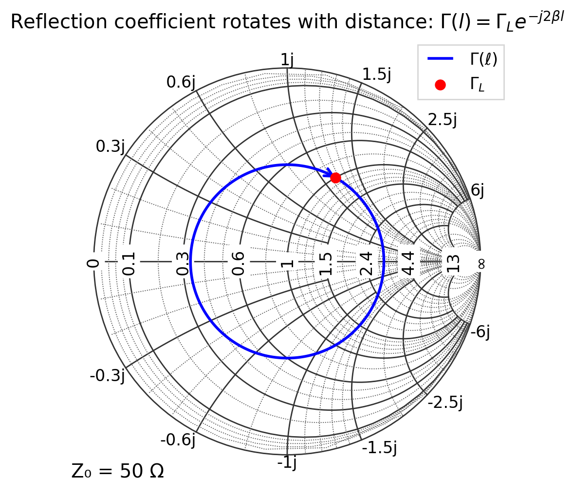
In R_DOMAIN, the Smith chart data are literally \(\Gamma\). So moving along the line is a simple complex rotation.
We start with a load reflection coefficient \(\Gamma_L\) and rotate it by a sequence of electrical lengths.
[2]:
Gamma_L = 0.5 * np.exp(1j * np.deg2rad(60))  # example load reflection coefficient
ell_over_lambda = np.linspace(0, 0.5, 201)  # 0 to half-wavelength

# Toward generator: Gamma(l) = Gamma_L * exp(-j 4 pi (ell/lambda))
Gamma = Gamma_L * np.exp(-1j * 4 * np.pi * ell_over_lambda)

plt.figure(figsize=(6, 6))
ax = plt.subplot(111, projection="smith", domain=R_DOMAIN)

ax.plot(Gamma, "b", label=r"$\Gamma(\ell)$", arrow="end")
ax.scatter(Gamma_L, c="r", s=50, label=r"$\Gamma_L$")

ax.legend(loc="upper right")
ax.set_title(r"Reflection coefficient rotates with distance: $\Gamma(l)=\Gamma_L e^{-j2\beta l}$")
plt.show()
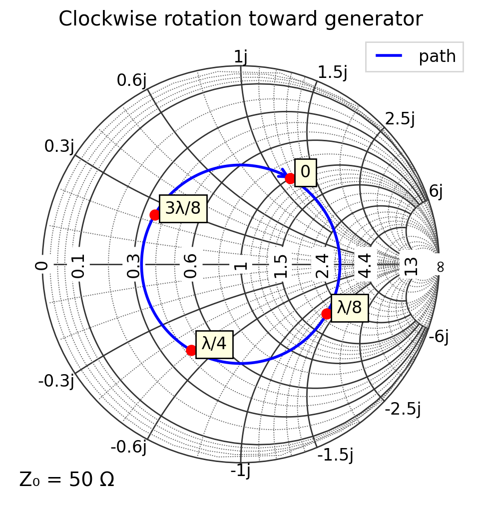
Direction: toward generator is clockwise
If we parameterize \(l\) increasing from the load toward the generator, the exponential term \(e^{-j2\beta l}\) rotates clockwise.
We will label a few points at eighth-wave intervals.
[9]:
Gamma_L = 0.5 * np.exp(1j * np.deg2rad(60))  # example load reflection coefficient
ell_over_lambda = np.linspace(0, 0.5, 201)  # 0 to half-wavelength
Gamma = Gamma_L * np.exp(-1j * 4 * np.pi * ell_over_lambda)

plt.figure(figsize=(6, 6))
ax = plt.subplot(111, projection="smith", domain=R_DOMAIN)

ax.plot(Gamma, "b", label="path", arrow="end")

text_offset = 0.05 + 0.03j
for frac, label in [(0.0, "0"), (0.125, "λ/8"), (0.25, "λ/4"), (0.375, "3λ/8")]:
    Gp = Gamma_L * np.exp(-1j * 4 * np.pi * frac)
    ax.scatter(Gp, c="r", s=50)
    ax.text(Gp + text_offset, label, bbox=text_box, zorder=10, va="center")

ax.legend(loc="upper right")
ax.set_title("Clockwise rotation toward generator")
plt.show()
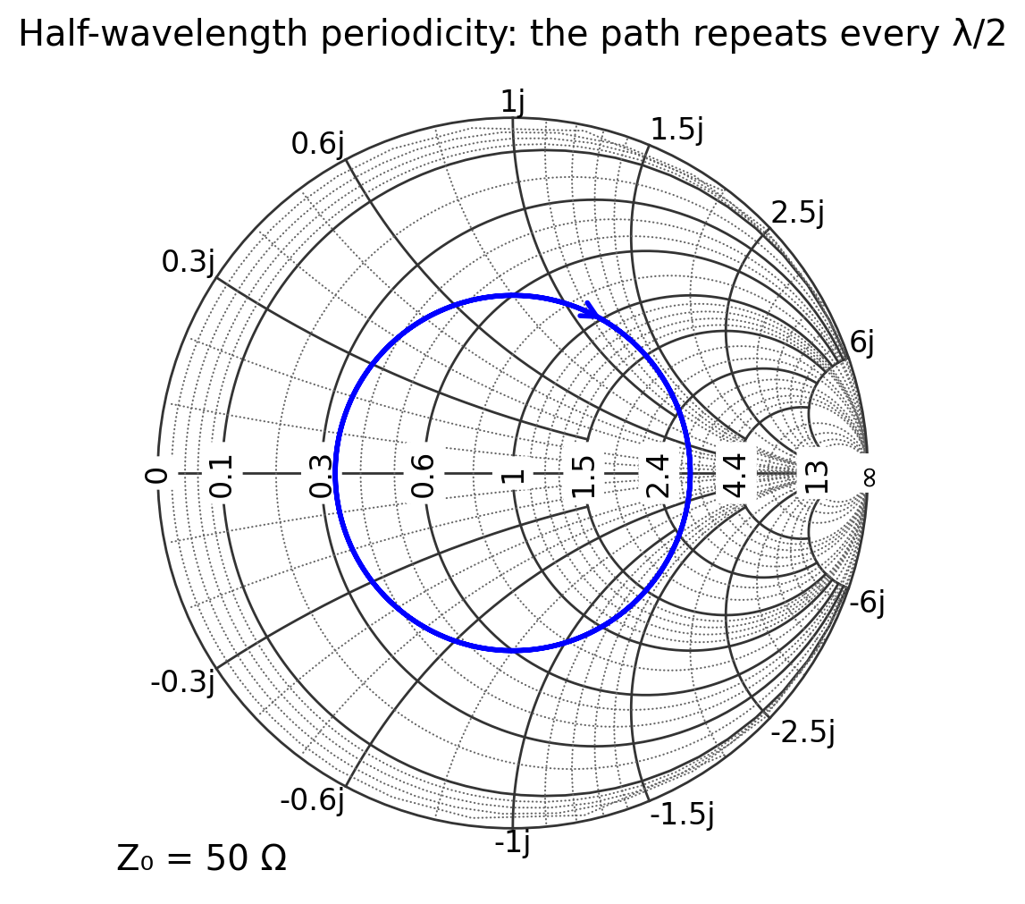
Half-wavelength periodicity
Because the phase rotation is \(2\beta \ell\), moving by \(\lambda/2\) produces a \(2\pi\) phase change in \(\Gamma\):
So the impedance pattern repeats every half-wavelength along a lossless line.
We can show this by plotting \(\Gamma(\ell)\) from 0 to \(\lambda\), and noting the path is traced twice.
[10]:
l_over_lambda2 = np.linspace(0, 1.0, 401)
Gamma2 = Gamma_L * np.exp(-1j * 4 * np.pi * l_over_lambda2)

plt.figure(figsize=(6, 6))
ax = plt.subplot(111, projection="smith", domain=R_DOMAIN)

ax.plot(Gamma2, "b", arrow="end")
ax.set_title("Half-wavelength periodicity: the path repeats every λ/2")
plt.show()
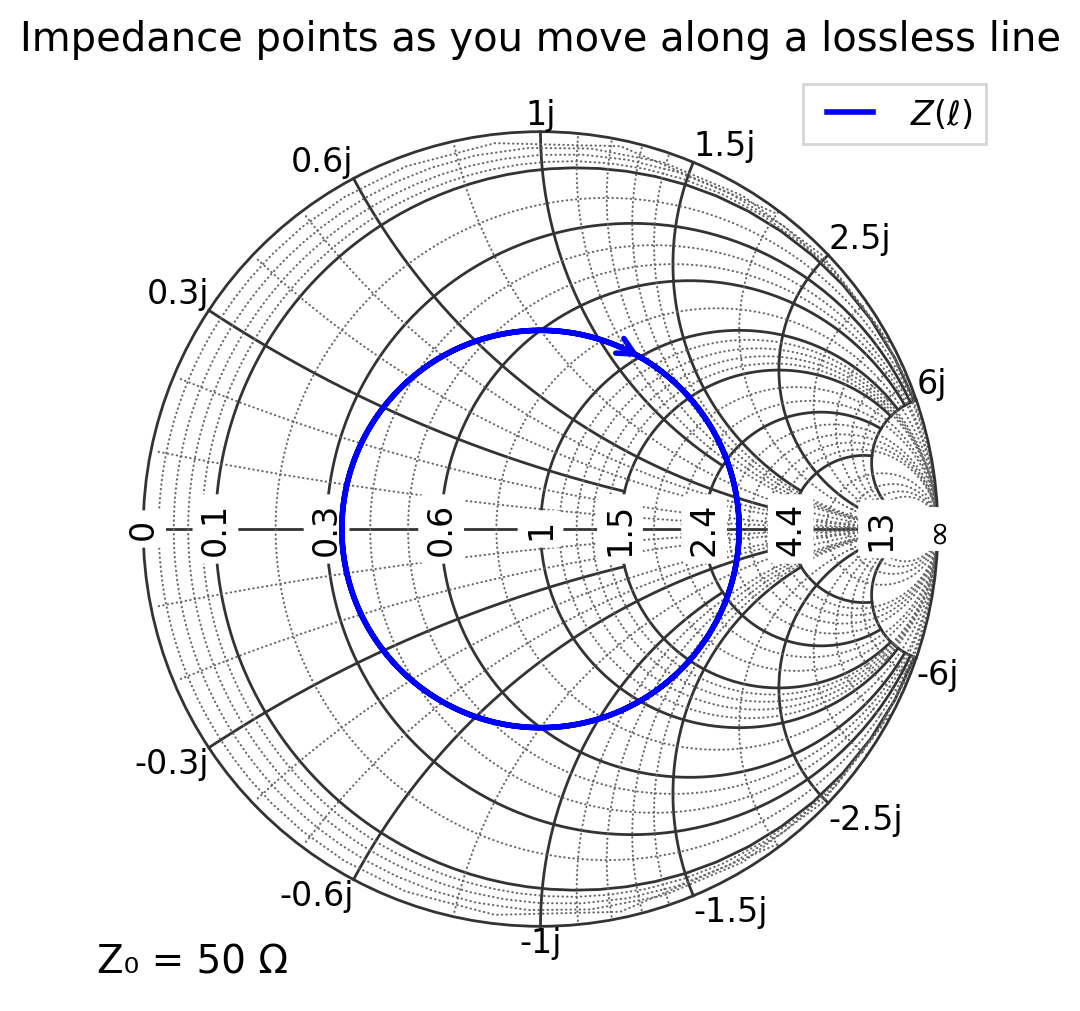
The same motion in impedance coordinates (Z_DOMAIN)
Many engineers think in terms of impedance \(Z\) rather than \(\Gamma\). We can convert \(\Gamma(\ell)\) into the corresponding input impedance:
In the default Z_DOMAIN, pysmithchart expects impedances in ohms and normalizes internally by \(Z_0\).
[11]:
Z0 = 50
l_over_lambda2 = np.linspace(0, 1.0, 401)
Gamma2 = Gamma_L * np.exp(-1j * 4 * np.pi * l_over_lambda2)
Z_in = utils.calc_load(Z0, Gamma2)

plt.figure(figsize=(6, 6))
ax = plt.subplot(111, projection="smith")

ax.plot(Z_in, "b", label=r"$Z(\ell)$", arrow="end")
ax.legend(loc="upper right")
ax.set_title("Impedance points as you move along a lossless line")
plt.show()
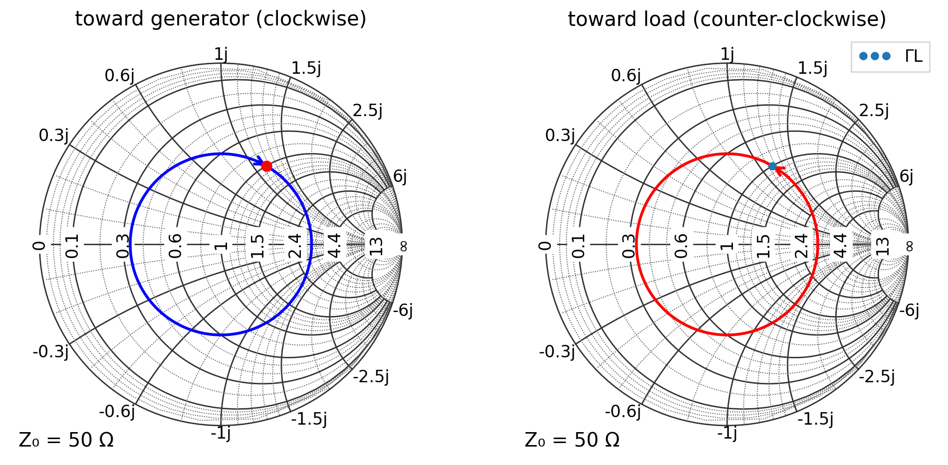
Rotate “toward generator” vs “toward load”
The sign convention matters.
Toward generator: \(\Gamma(l) = \Gamma_L e^{-j2\beta l}\)
Toward load: \(\Gamma(l) = \Gamma_L e^{+j2\beta l}\)
If your path appears to rotate the “wrong way,” check your direction and sign convention.
[6]:
Gamma_L = 0.5 * np.exp(1j * np.deg2rad(60))  # example load reflection coefficient
ell = np.linspace(0, 0.5, 201)

Gamma_toward_gen = Gamma_L * np.exp(-1j * 4 * np.pi * ell)
Gamma_toward_load = Gamma_L * np.exp(+1j * 4 * np.pi * ell)

plt.figure(figsize=(12, 6))
ax = plt.subplot(121, projection="smith", domain=R_DOMAIN)

ax.plot(Gamma_toward_gen, "b", arrow=True)
ax.scatter(Gamma_L, c="r", s=50)
ax.set_title("toward generator (clockwise)")

ax = plt.subplot(122, projection="smith", domain=R_DOMAIN)

ax.plot(Gamma_toward_load, "r", arrow=True)
ax.plot(Gamma_L, "o", label="ΓL")

ax.legend(loc="upper right")
ax.set_title("toward load (counter-clockwise)")
plt.show()
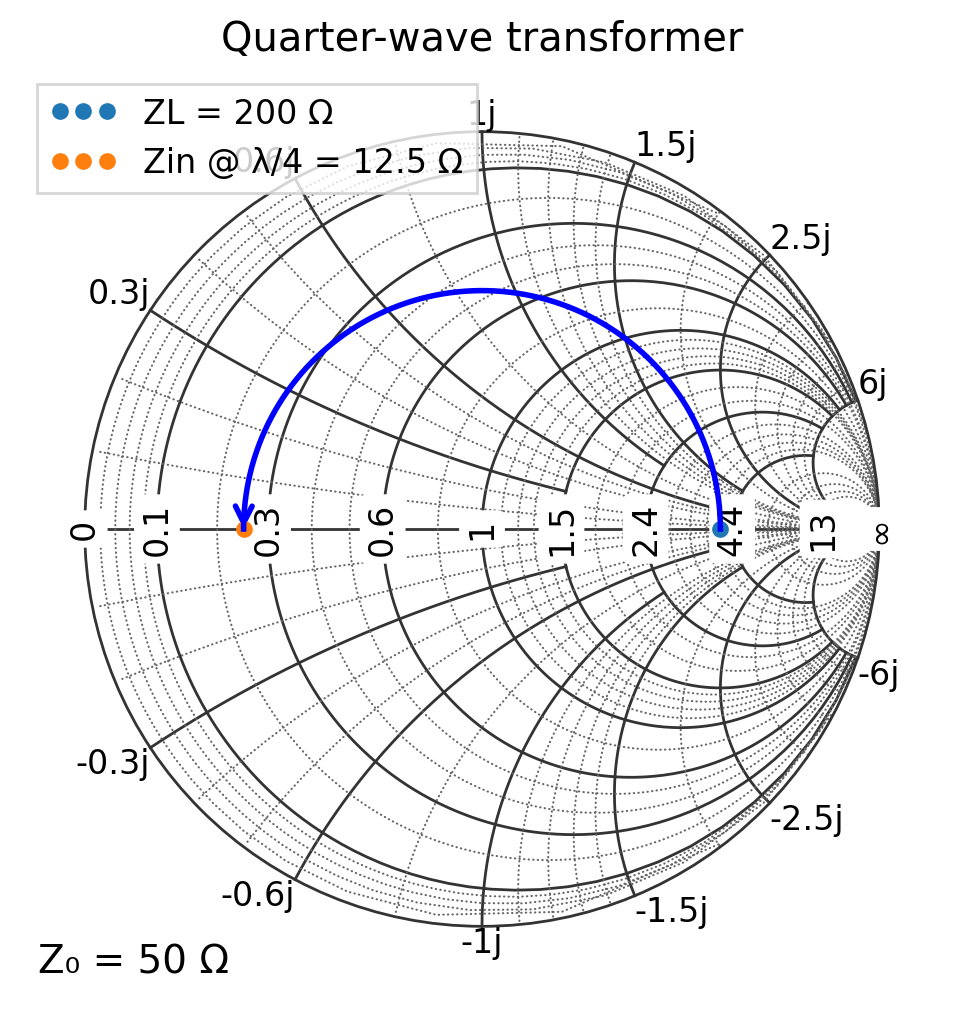
Quarter-wave transformer example
A classic result: a lossless quarter-wave section transforms impedances according to:
This is the special case of the general transmission-line input impedance formula when \(\ell=\lambda/4\).
We can compute this by rotating \(\Gamma\) by \(180^\circ\) (since \(2\beta(\lambda/4) = \pi\)) and converting back to impedance.
[7]:
Z0 = 50
ZL = 200 + 0j
Gamma_L = utils.calc_gamma(Z0, ZL)

# Quarter-wave toward generator: rotate Gamma by -pi
Gamma_qw = Gamma_L * np.exp(-1j * np.pi)
Zin_qw = utils.calc_load(Z0, Gamma_qw)

vswr = utils.calc_vswr(Z0, ZL)
plt.figure(figsize=(6, 6))
ax = plt.subplot(111, projection="smith")

ax.plot([ZL], "o", label=f"ZL = {ZL.real:.0f} Ω")
ax.plot([Zin_qw], "o", label=f"Zin @ λ/4 = {Zin_qw.real:.1f} Ω")
ax.plot_vswr(vswr, "b", angle_range=(0, 180), arrow="end")

ax.legend(loc="upper left")
ax.set_title("Quarter-wave transformer")
plt.show()
[ ]: