Smith chart domains
pysmithchart can plot several different domains on the same Smith chart projection. The domain determines what you pass to ax.plot() / ax.scatter() / ax.text() and how the library converts that data internally for display.
This notebook explains each domain and shows small, self-contained examples.
[1]:
%config InlineBackend.figure_format = 'retina'

import sys
import numpy as np
import matplotlib.pyplot as plt

if sys.platform == "emscripten":
    import piplite

    await piplite.install("pysmithchart")

import pysmithchart
from pysmithchart import Z_DOMAIN, Y_DOMAIN, R_DOMAIN, NORM_Z_DOMAIN, NORM_Y_DOMAIN
from pysmithchart import utils

text_box = dict(facecolor="lightyellow")
Domain quick reference
The Smith chart itself is drawn in terms of normalized impedance
but users naturally work with different quantities (ohms, siemens, reflection coefficient). pysmithchart supports these through a domain= choice.
Domain constant |
What you pass to plotting calls |
Internal conversion |
Typical use |
|---|---|---|---|
|
\(Z\) in ohms |
\(z = Z/Z_0\) |
Most RF matching, measured impedances |
|
\(z\) normalized (dimensionless) |
use as-is |
data matches impedance grid |
|
\(\Gamma\) (a.k.a. S11), complex |
\(z = (1+\Gamma)/(1-\Gamma)\) |
VNAs / S-parameter workflows |
|
\(Y\) in siemens |
\(z = \frac{1}{Y Z_0}\) |
Admittance-based matching, dual networks |
|
\(y\) normalized (dimensionless) |
use as-is |
data matches admittance grid |
Domains let you supply the quantity you naturally have: \(Z\), \(z\), \(Y\), or \(\Gamma\).
How to set the domain
You can reset the default domain for all subsequent plots on an axis:
ax = plt.subplot(111, projection="smith", domain=NORM_Z_DOMAIN)
or per plotting call (overrides the default):
ax.plot(Γ, domain=R_DOMAIN)
ax.text(z.real, z.imag, "label", domain=Z_DOMAIN)
A single physical load shown four ways
We will use the same physical load, and plot it using each domain.
Reference impedance:
Z0 = 50 ΩLoad impedance:
ZL = 25 + j25 Ω
From these we can compute:
normalized impedance:
z = ZL / Z0admittance:
Y = 1 / ZLreflection coefficient:
Γ = (ZL - Z0) / (ZL + Z0)
[2]:
Z0 = 50
ZL = 30 + 1j * 30

z_norm = ZL / Z0
Y = 1 / ZL
Gamma = utils.calc_gamma(Z0, ZL)

print("ZL =", ZL)
print("z  =", z_norm)
print("Y  =", utils.cs(Y, 3))
print("Γ  =", utils.cs(Gamma, 3))
ZL = (30+30j)
z  = (0.6+0.6j)
Y  =  0.017 -  0.017j
Γ  = -0.096 +  0.411j
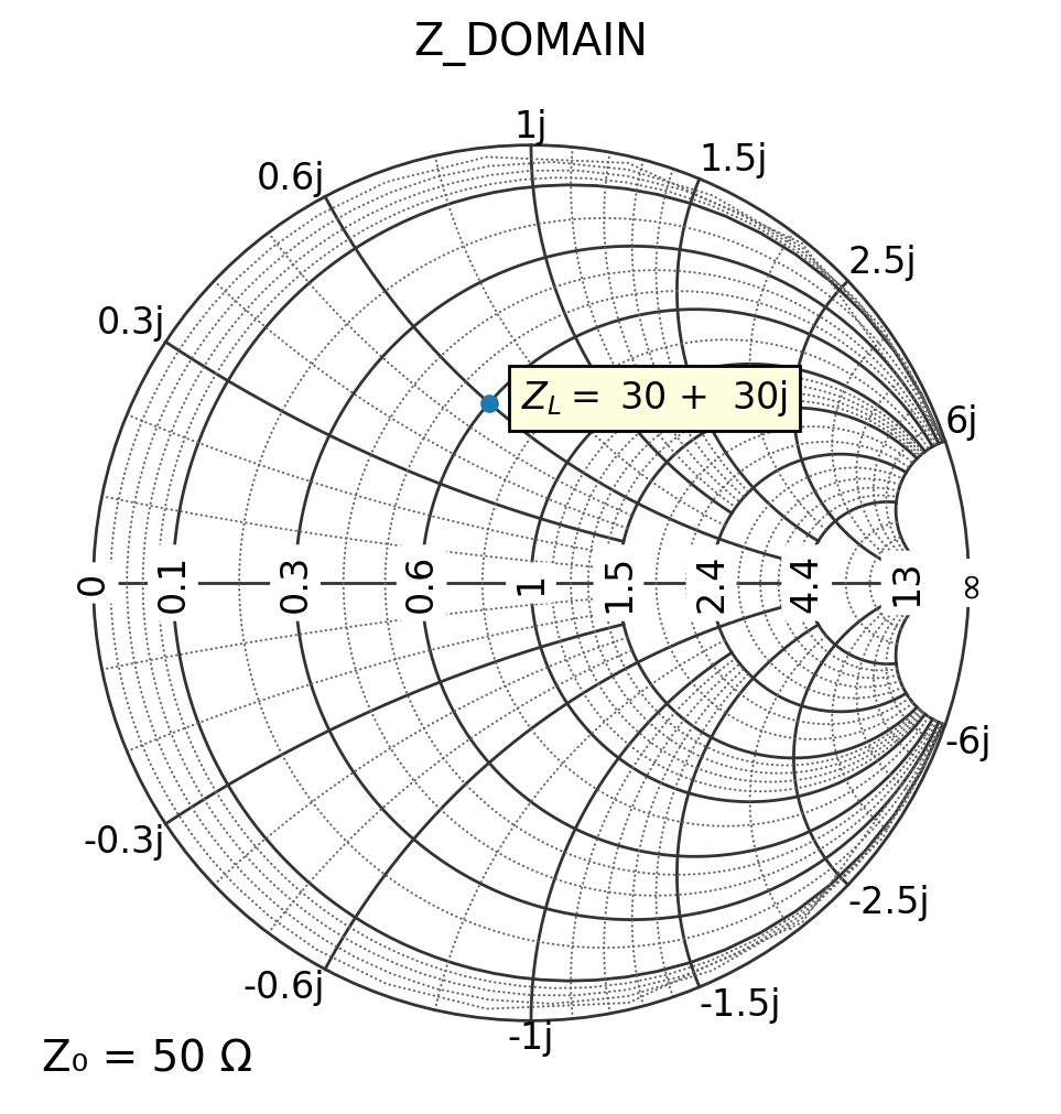
1) Z_DOMAIN: pass ohms
This is the default domain. You pass Z in ohms; pysmithchart divides by Z0 internally.
[3]:
plt.figure(figsize=(6, 6))
ax = plt.subplot(111, projection="smith", Z0=Z0)

ax.plot(ZL, marker="o", linestyle="")
text_offset = 5 + 3j
ax.text(ZL + text_offset, "$Z_L =$" + utils.cs(ZL, 0), bbox=text_box)

ax.set_title("Z_DOMAIN")
plt.show()
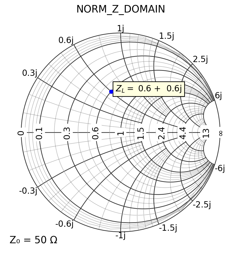
2) NORM_Z_DOMAIN: pass normalized z (dimensionless)
In this domain, you pass z = Z/Z0 directly. These values should appear just where you expect them on the chart
[4]:
Z0 = 50
ZL = 30 + 1j * 30
z_norm = ZL / Z0

plt.figure(figsize=(6, 6))
ax = plt.subplot(111, projection="smith", domain=NORM_Z_DOMAIN)

ax.plot(z_norm, "bo")
text_offset = 0.05 + 0.05j
ax.text(z_norm + text_offset, "$Z_L =$" + utils.cs(z_norm, 2), bbox=text_box)

ax.set_title("NORM_Z_DOMAIN")
plt.show()
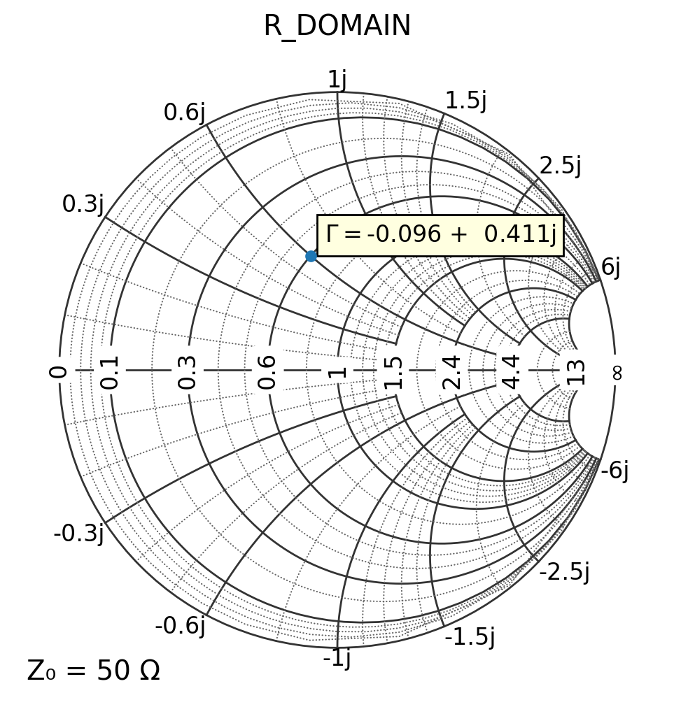
3) R_DOMAIN: pass Γ (S11)
If you have S-parameters from a VNA or simulator, you might start with Γ directly. In the R_DOMAIN pysmithchart internally converts the datapoint to normalized impedance using the inverse Möbius transform:
Only points inside the unit circle |Γ| ≤ 1 are visible on the chart.
[5]:
Z0 = 50
ZL = 30 + 1j * 30
Gamma = utils.calc_gamma(Z0, ZL)

plt.figure(figsize=(6, 6))
ax = plt.subplot(111, projection="smith", domain=R_DOMAIN)

ax.plot(Gamma, marker="o", linestyle="")
text_offset = 0.05 + 0.05j
ax.text(Gamma + text_offset, "$\Gamma =$" + utils.cs(Gamma, 3), bbox=text_box)

ax.set_title("R_DOMAIN")
plt.show()
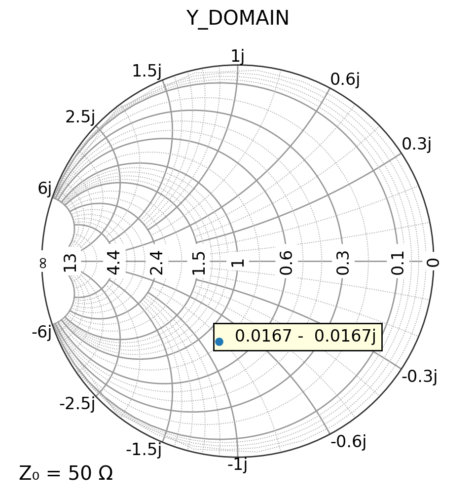
4) Y_DOMAIN: pass Y in siemens
Admittance plotting is useful for “dual” matching workflows (e.g., shunt elements).
Internally, pysmithchart converts Y to normalized impedance using: \(z = \frac{1}{Y Z_0}\)
[6]:
ZL = 30 + 1j * 30
YL = 1 / ZL

plt.figure(figsize=(6, 6))
ax = plt.subplot(111, projection="smith", grid="admittance", domain=Y_DOMAIN)

ax.plot(YL, marker="o", linestyle="")
ax.text(YL, "  " + utils.cs(YL, 4), bbox=text_box)

ax.set_title("Y_DOMAIN")
plt.show()
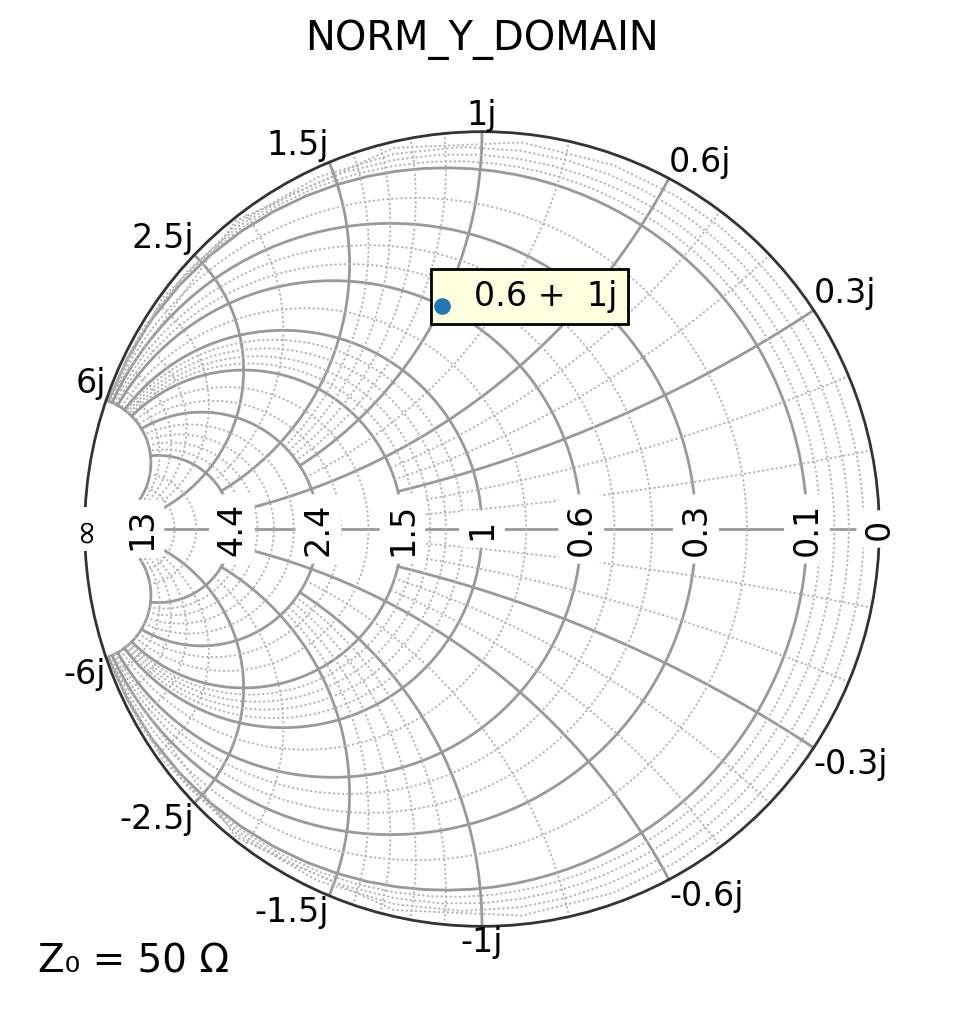
5) NORM_Y_DOMAIN: pass normalized admittance (dimensionless)**
Admittance plotting is useful for “dual” matching workflows (e.g., shunt elements).
[7]:
y = 0.6 + 1j

plt.figure(figsize=(6, 6))
ax = plt.subplot(111, projection="smith", grid="admittance", domain=NORM_Y_DOMAIN)

ax.plot(y, marker="o", linestyle="")
ax.text(y, "  " + utils.cs(y, 4), bbox=text_box)

ax.set_title("NORM_Y_DOMAIN")
plt.show()
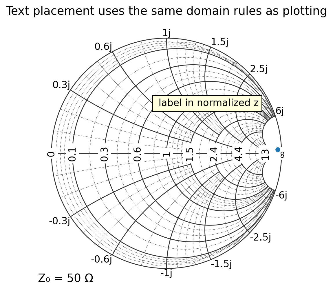
What about ax.text() and ax.annotate()?
pysmithchart applies the same domain logic to text() and annotate() as it does to plot().
All forms below work fine in all four domains
ax.text(z, label, ...)ax.text(x, y, label, ...)ax.annotate(x, y, label, ...)
Note because annotate has two positions xy and xytext, you cannot use complex values with annotate
A simple example of ax.text()
[8]:
Z0 = 50
ZL = 30 + 1j * 30
z_norm = ZL / Z0

plt.figure(figsize=(6, 6))
ax = plt.subplot(111, projection="smith", domain=NORM_Z_DOMAIN)

ax.plot(ZL, marker="o", linestyle="")
ax.text(z_norm, " label in normalized z", bbox=text_box)

ax.set_title("Text placement uses the same domain rules as plotting")
plt.show()
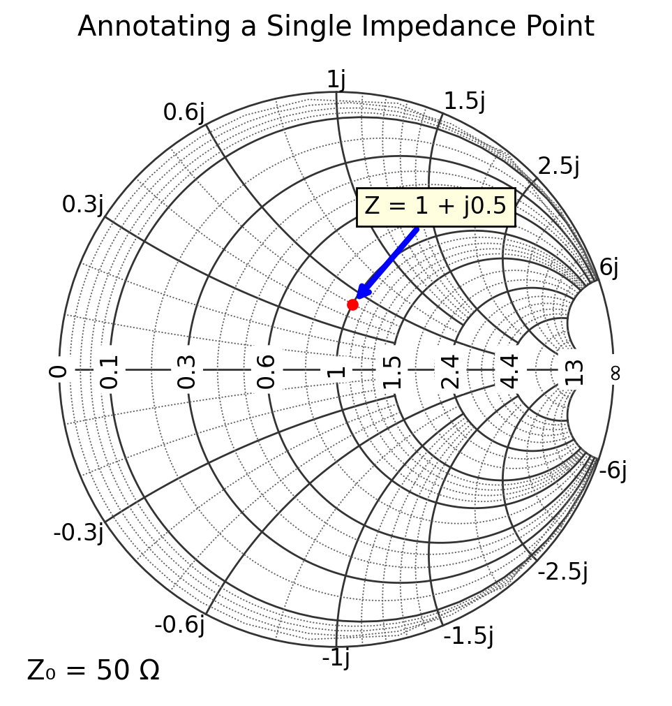
A simple example of ax.annotate()
[9]:
plt.figure(figsize=(6, 6))
ax = plt.subplot(111, projection="smith", domain=NORM_Z_DOMAIN)

z = 1 + 0.5j
ax.plot(z, "ro")

# Annotate the point
ax.annotate(
    "Z = 1 + j0.5",
    xy=(z.real, z.imag),  # point being annotated (Smith coords)
    xytext=(0.6, 1.0),  # location of text
    arrowprops=dict(arrowstyle="->", color="blue", lw=3),
    bbox=text_box,
)

ax.set_title("Annotating a Single Impedance Point")
plt.show()
[ ]: