Arrow Support in Smith Charts
This notebook demonstrates the arrow functionality available in pysmithchart for visualizing direction and flow on Smith charts.
Arrow support is available in:
plot()- Main plotting functionplot_constant_resistance()- Resistance circlesplot_constant_reactance()- Reactance arcsplot_constant_conductance()- Conductance circles (admittance)plot_constant_susceptance()- Susceptance arcs (admittance)plot_vswr()- VSWR circlesplot_rotation_path()- Matching paths
[1]:
%config InlineBackend.figure_format = 'retina'

import sys
import numpy as np
import matplotlib.pyplot as plt

if sys.platform == "emscripten":
    import piplite

    await piplite.install("pysmithchart")

from pysmithchart import R_DOMAIN, Z_DOMAIN, Y_DOMAIN, NORM_Y_DOMAIN, NORM_Z_DOMAIN
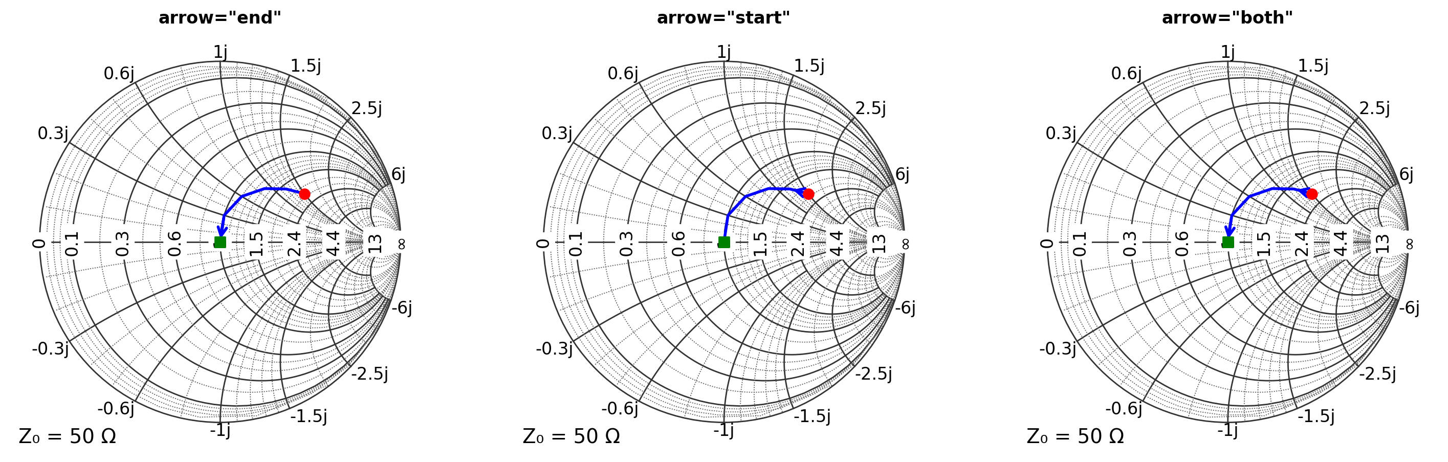
Basic Arrow Usage with ax.plot()
The simplest way to add arrows is with the arrow parameter.
[2]:
Z = np.array([100 + 75j, 80 + 60j, 65 + 45j, 55 + 30j, 50 + 15j, 50 + 0j])

plt.figure(figsize=(18, 6))

# Arrow at end
ax = plt.subplot(131, projection="smith")
ax.plot(Z, "b", linewidth=2, arrow="end")
ax.scatter(Z[0], c="red", s=50, marker="o", label="Start", zorder=10)
ax.scatter(Z[-1], c="green", s=50, marker="s", label="End", zorder=10)
ax.set_title('arrow="end"', fontsize=12, fontweight="bold")

# Arrow at start
ax = plt.subplot(132, projection="smith")
ax.plot(Z, "b", linewidth=2, arrow="start")
ax.scatter(Z[0], c="red", s=50, marker="o", label="Start", zorder=10)
ax.scatter(Z[-1], c="green", s=50, marker="s", label="End", zorder=10)
ax.set_title('arrow="start"', fontsize=12, fontweight="bold")

# Arrows at both ends
ax = plt.subplot(133, projection="smith")
ax.plot(Z, "b", linewidth=2, arrow="both")
ax.scatter(Z[0], c="red", s=50, marker="o", label="Start")
ax.scatter(Z[-1], c="green", s=50, marker="s", label="End")
ax.set_title('arrow="both"', fontsize=12, fontweight="bold")

plt.show()
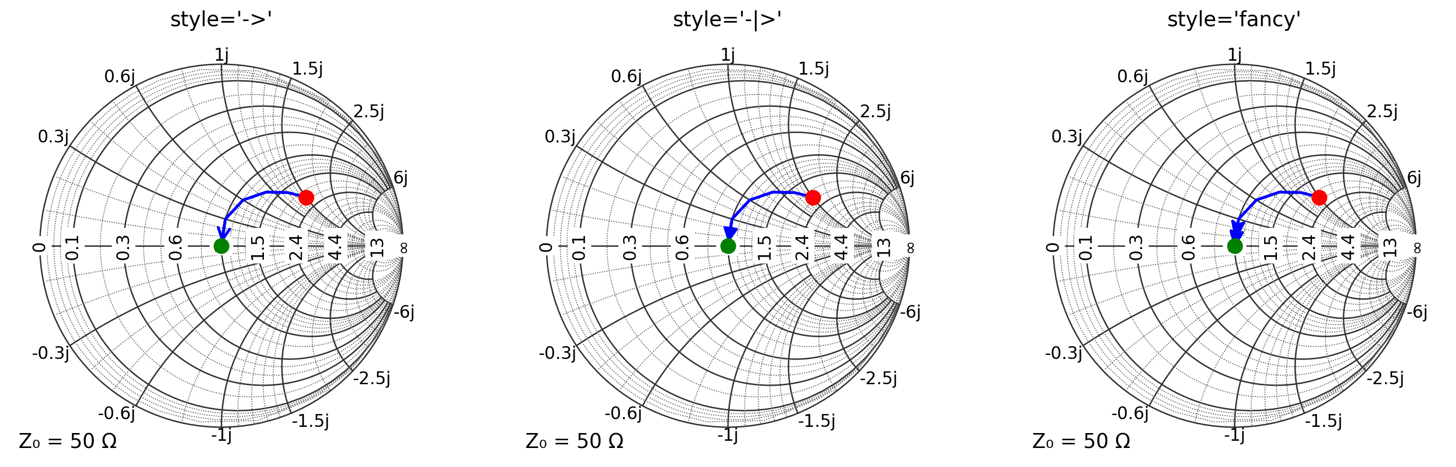
Custom Arrow Styles
Use a dictionary for full control over arrow appearance.
[3]:
Z = np.array([100 + 75j, 80 + 60j, 65 + 45j, 55 + 30j, 50 + 15j, 50 + 0j])

arrow_styles = [("->", "Standard"), ("-|>", "Fancy"), ("fancy", "Fancy Arrow")]

plt.figure(figsize=(18, 6))
for i, tuple in enumerate(arrow_styles):
    style, name = tuple
    arrow_dict = {"position": "end", "style": style, "size": 20}
    ax = plt.subplot(1, 3, i + 1, projection="smith")
    ax.plot(Z, "b-", linewidth=2, arrow=arrow_dict)
    ax.scatter(Z[0], c="red", s=100, marker="o")
    ax.scatter(Z[-1], c="green", s=100, marker="o")
    ax.set_title(f"style='{style}'")

plt.show()
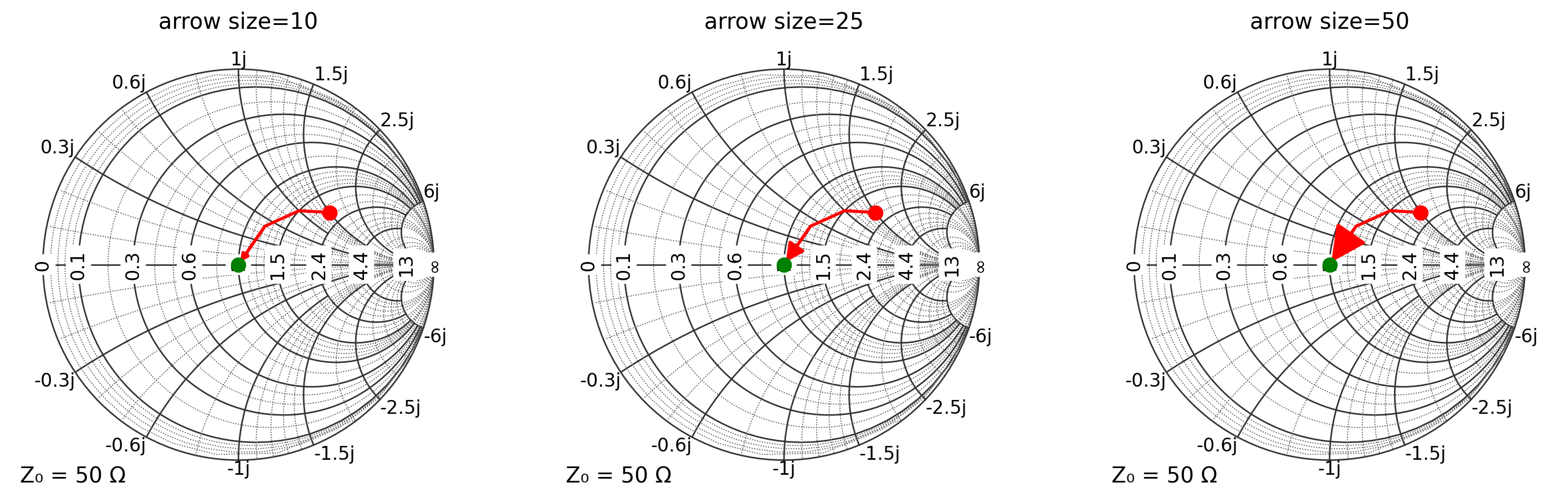
Arrow Size Control
Adjust arrow size for visibility and aesthetics.
[4]:
Z = np.array([100 + 75j, 75 + 50j, 60 + 25j, 50 + 0j])
sizes = [10, 25, 50]

plt.figure(figsize=(18, 6))
for i, size in enumerate(sizes):
    arrow_dict = {"position": "end", "style": "-|>", "size": size}
    ax = plt.subplot(1, 3, i + 1, projection="smith")
    ax.plot(Z, "r-", linewidth=2, arrow=arrow_dict)
    ax.scatter(Z[0], c="red", s=80, marker="o")
    ax.scatter(Z[-1], c="green", s=80, marker="o")
    ax.set_title(f"arrow size={size}")
plt.show()
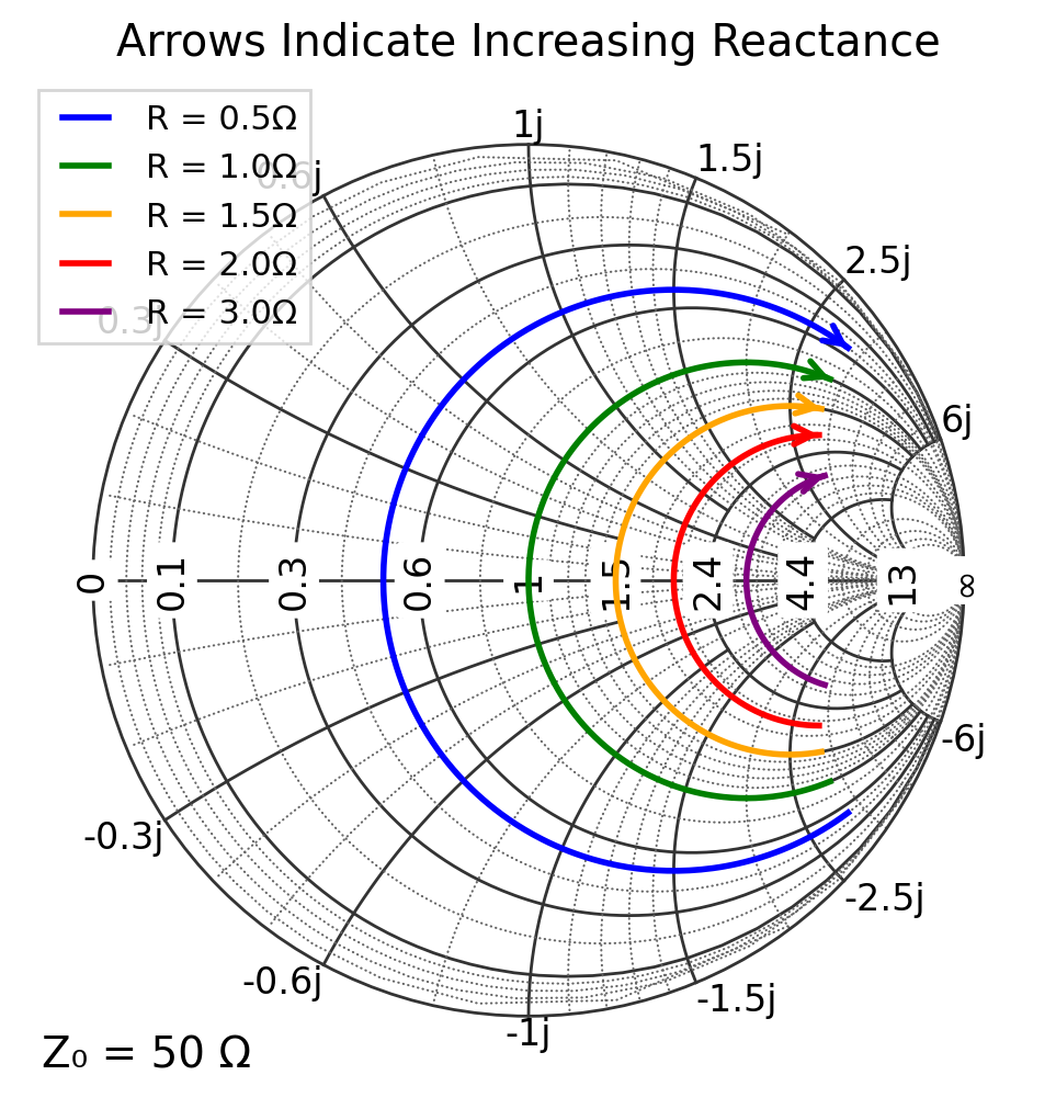
Arrows on Constant Resistance Circles
Show increasing reactance direction on resistance circles. He we range from -150j to +150j (or normalized from -3j to +3j).
[5]:
Z0 = 50
plt.figure(figsize=(6, 6))
ax = plt.subplot(111, projection="smith")

norm_resistances = np.array([25, 50, 75, 100, 150]) / Z0
colors = ["blue", "green", "orange", "red", "purple"]

for r, color in zip(norm_resistances, colors):
    ax.plot_constant_resistance(r, c=color, ms=0, ls="-", lw=2, range=(-3, 3), arrow="end", label=f"R = {r}Ω")

ax.legend(loc="upper left", fontsize=11)
ax.set_title("Arrows Indicate Increasing Reactance")
plt.show()
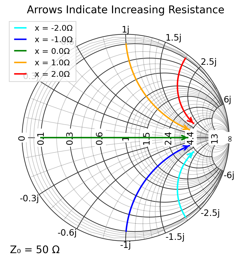
Arrows on Constant Reactance Arcs
Show increasing resistance direction on reactance arcs.
[6]:
Z0 = 50
plt.figure(figsize=(6, 6))
ax = plt.subplot(111, projection="smith")

norm_reactances = np.array([-100, -50, 0, 50, 100]) / Z0
colors = ["cyan", "blue", "green", "orange", "red"]

for x, color in zip(norm_reactances, colors):
    label = f"x = {x}Ω"
    ax.plot_constant_reactance(x, c=color, ms=0, ls="-", lw=2, range=(0.1, 4), arrow="end", label=label)

ax.legend(loc="upper left", fontsize=11)
ax.set_title("Arrows Indicate Increasing Resistance")
plt.show()
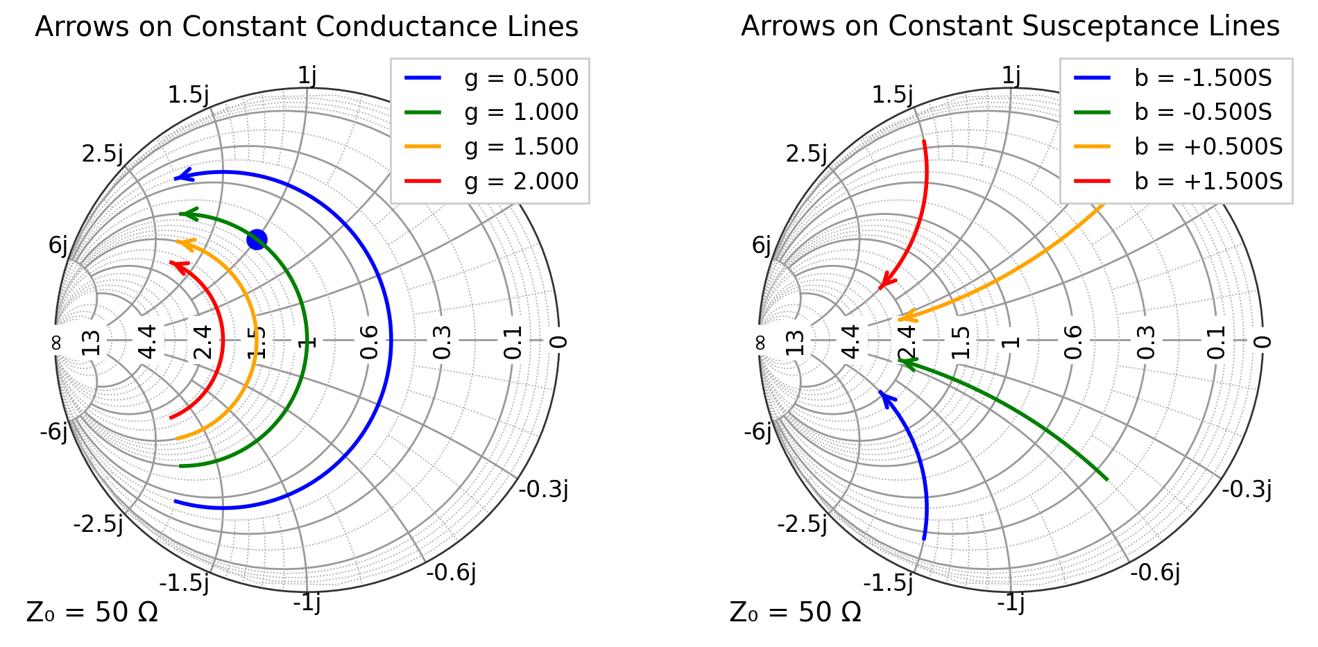
Admittance Arrows
Arrows work on admittance lines too!
[7]:
Z0 = 50
Y0 = 1 / Z0
norm_conductances = np.array([0.01, 0.02, 0.03, 0.04]) / Y0
norm_susceptances = np.array([-0.03, -0.01, 0.01, 0.03]) / Y0
colors = ["blue", "green", "orange", "red"]

r1 = (-0.04 / Y0, 0.04 / Y0)
r2 = (0.005 / Y0, 0.05 / Y0)
plt.figure(figsize=(12, 6))

# Plot constant conductance arcs
ax = plt.subplot(121, projection="smith", grid="admittance")
ax.scatter(1 + 1j, c="blue", s=100, domain=NORM_Y_DOMAIN)
for g, color in zip(norm_conductances, colors):
    s = f"g = {g:.3f}"
    ax.plot_constant_conductance(g, c=color, ms=0, lw=2, range=r1, arrow="end", label=s)
ax.legend(loc="upper right", framealpha=1)
ax.set_title("Arrows on Constant Conductance Lines")

# Plot constant susceptance arcs
ax = plt.subplot(122, projection="smith", grid="admittance")
for b, color in zip(norm_susceptances, colors):
    s = f"b = {b:+.3f}S"
    ax.plot_constant_susceptance(b, c=color, ms=0, lw=2, range=r2, arrow="end", label=s)

ax.legend(loc="upper right", framealpha=1)
ax.set_title("Arrows on Constant Susceptance Lines")
plt.show()
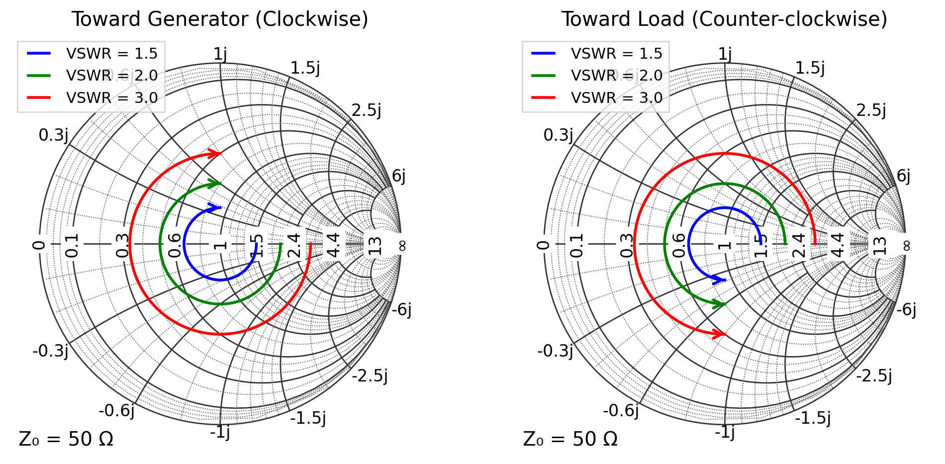
Arrows on VSWR Circles
Show rotation direction along transmission line.
[8]:
plt.figure(figsize=(12, 6))

vswr_values = [1.5, 2.0, 3.0]
colors = ["blue", "green", "red"]

# Clockwise rotation (toward generator)
ax = plt.subplot(121, projection="smith")
for vswr, color in zip(vswr_values, colors):
    ax.plot_vswr(vswr, color=color, ms=0, ls="-", lw=2, angle_range=(0, -270), arrow="end", label=f"VSWR = {vswr}")

ax.legend(loc="upper left", fontsize=11)
ax.set_title("Toward Generator (Clockwise)")

# Counter-clockwise rotation (toward load)
ax = plt.subplot(122, projection="smith")
for vswr, color in zip(vswr_values, colors):
    ax.plot_vswr(vswr, color=color, ms=0, ls="-", lw=2, angle_range=(0, 270), arrow="end", label=f"VSWR = {vswr}")

ax.legend(loc="upper left", fontsize=11)
ax.set_title("Toward Load (Counter-clockwise)")
plt.show()
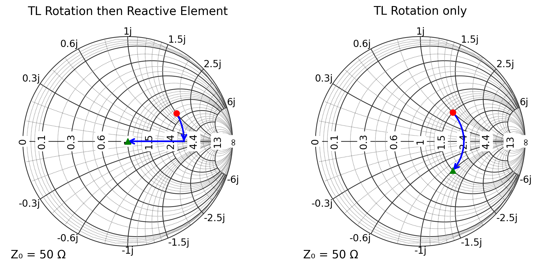
Arrows on Matching Paths
Visualize impedance matching networks with directional arrows.
[9]:
Z_load = 100 + 75j
Z_matched = 50 + 0j

plt.figure(figsize=(12, 6))
ax = plt.subplot(121, projection="smith")
ax.plot_rotation_path(Z_load, Z_matched, "b-", linewidth=2, arrow="end")
ax.scatter(Z_load, c="red", s=50, marker="o")
ax.scatter(Z_matched, c="green", s=50, marker="^")
ax.set_title("TL Rotation then Reactive Element")

Z_load = 75 + 50j
Z_matched = 75 - 50j  # Same VSWR

ax = plt.subplot(122, projection="smith")
ax.plot_rotation_path(Z_load, Z_matched, "b-", linewidth=2, arrow="end")
ax.scatter(Z_load, c="red", s=50, marker="o")
ax.scatter(Z_matched, c="green", s=50, marker="^")
ax.set_title("TL Rotation only")
plt.show()
[ ]: