Quickstart

This notebook shows the minimum you need to:

• Create a Matplotlib axis with the Smith chart projection.

• Plot a few impedances on the chart.

• Add labels with ax.text().

Defaults:

• Default plotting is in the impedance domain with datapoints in ohms.

• The default characteristic impedance is \(Z_0=50 \Omega\).

• pysmithchart normalizes internally by the characteristic impedance \(Z_0\).

%config InlineBackend.figure_format = 'retina'

import sys
import numpy as np
import matplotlib.pyplot as plt

if sys.platform == "emscripten":
    import piplite

    await piplite.install("pysmithchart")

# Importing pysmithchart registers the "smith" Matplotlib projection.
import pysmithchart

Create a Smith chart axis

The best way to set up Matplotlib to use the Smith (Möbius) transform is:

plt.figure(figsize=(6, 6))
ax = plt.subplot(111, projection="smith")

The example below creation of the plot and automatic generation of Smith chart gridlines.

In general, impedances are complex numbers. The simplest way to plot with pysmithchart is to pass the complex numbers as values. The default expectation is that all numbers you supply should be unnormalized impedances in ohms.

You can pass complex values directly to ax.plot(...), ax.scatter(...), ax.annotate(...), and ax.text(...)

You might be concerned the usual plot call in matplotlib requires both x and y values, i.e., ax.plot(x,y) `pysmithplot converts the complex impedance values to real and imaginary components internally. Two element plotting is still available if you do ax.plot(z.imag, z.real)

Z = [
    50 + 0j,  # matched load
    100 + 0j,  # higher resistance
    25 + 0j,  # lower resistance
    50 + 50j,  # inductive
    50 - 50j,  # capacitive
]
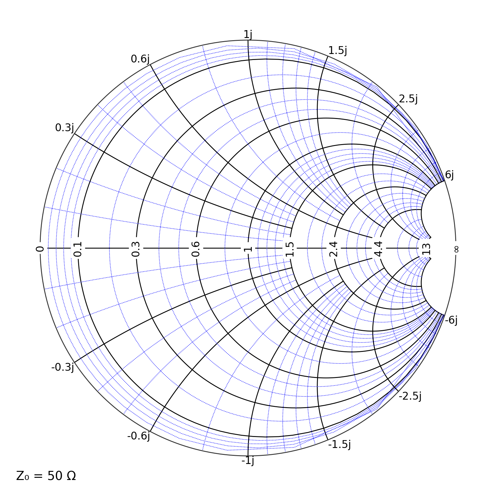
sc = {"grid.Z.major.color": "black", "grid.Z.minor.color": "blue"}
# two line setup for graph
plt.figure(figsize=(10, 10))
ax = plt.subplot(111, projection="smith", **sc)

# plot the points
# ax.scatter(Z, s=60, color="red")
plt.savefig("sc.svg", bbox_inches="tight")
plt.show()

Changing the default characteristic impedance

In the default impedance domain, you supply impedances in ohms, and pysmithchart normalizes internally by Z₀.

• If your system is 50 Ω (common in RF), you can use the default.

• If you want a different Z₀, pass it when creating the axes.

Examples:

ax = plt.subplot(111, projection="smith")                 # default Z0 = 50Ω
ax = plt.subplot(111, projection="smith", Z0=75)          # change Z0 to 75Ω

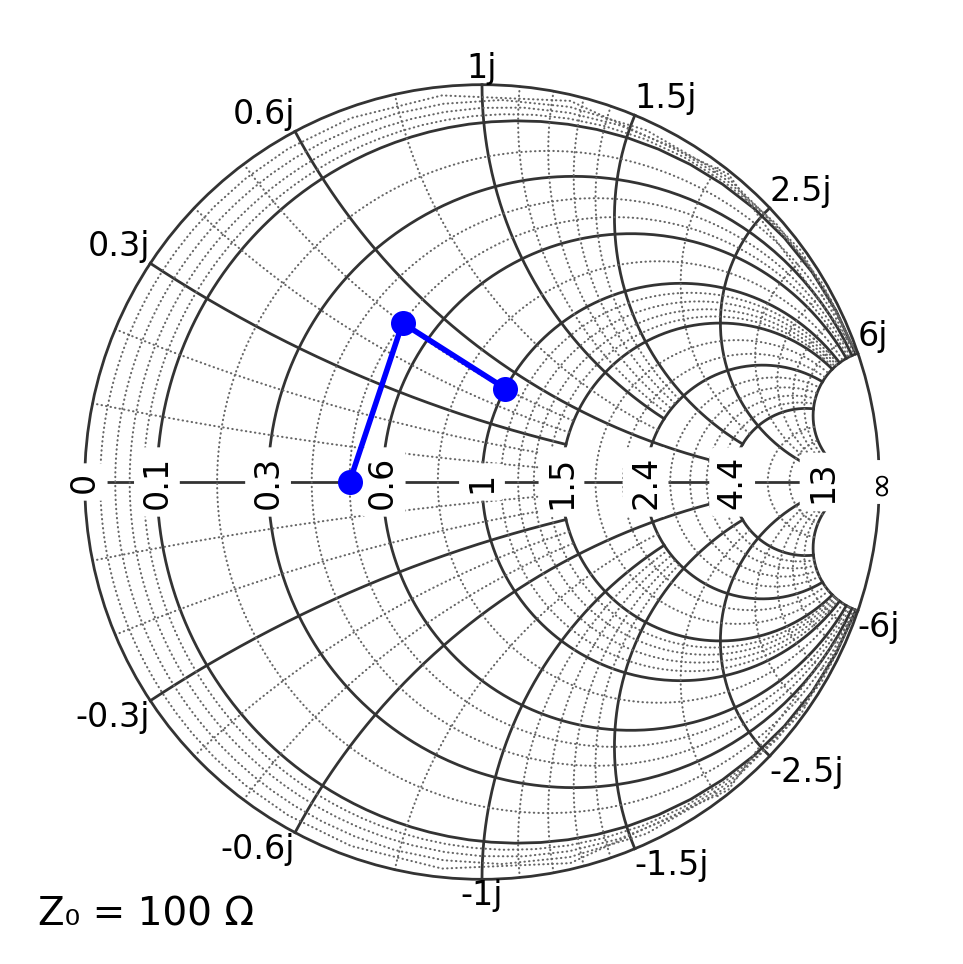
The example below illustrates an array of impedances can be plotted at once.

Z = [50 + 0j, 50 + 50j, 100 + 50j]

plt.figure(figsize=(6, 6))
ax = plt.subplot(111, projection="smith", Z0=100)  # set Z0 = 100 Ω
ax.plot(Z, "bo-", ms=8)
plt.show()

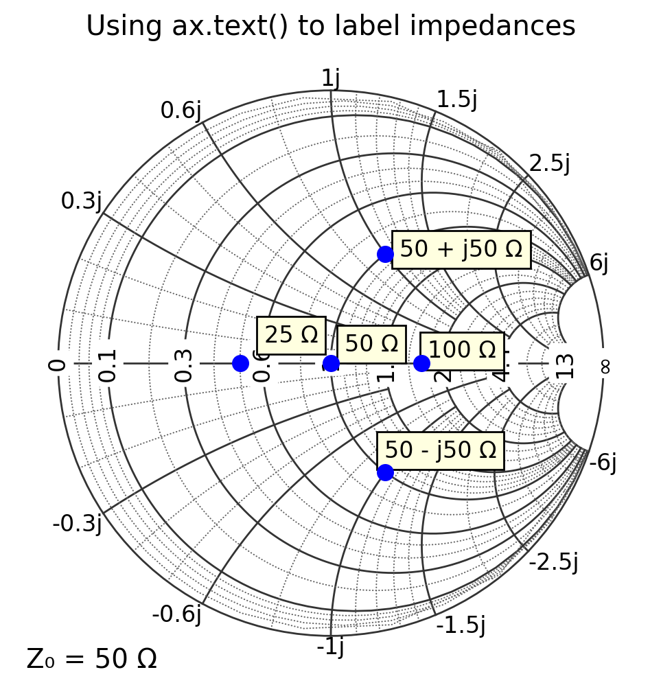
Adding labels with ax.text()

Use ax.text(z, "label", ...) to place text next to the point Z in Smith chart.

Important: on a Smith chart, the displayed (screen) coordinates are not the same as the data coordinates. For pysmithchart, the data coordinates represent the complex quantity you are plotting in the selected domain:

• In the default impedance domain, x and y correspond to \(\Re\{Z\}\) and \(\Im\{Z\}\) in ohms.

A practical trick is to apply a small offset (still in the same domain coordinates) so labels do not sit directly on markers.

text_box = {"facecolor": "lightyellow", "edgecolor": None}

plt.figure(figsize=(6, 6))
ax = plt.subplot(111, projection="smith")  # default Z0 = 50 Ω

Z0 = 50
Z = np.array([Z0 + 0j, 2 * Z0 + 0j, 0.5 * Z0 + 0j, Z0 + 1j * Z0, Z0 - 1j * Z0])
labels = ["50 Ω", "100 Ω", "25 Ω", "50 + j50 Ω", "50 - j50 Ω"]

ax.plot(Z, "bo", ms=8, ls="")

text_offset = 5 + 5j
for Zi, s in zip(Z, labels):
    ax.text(Zi + text_offset, s, bbox=text_box)

ax.set_title("Using ax.text() to label impedances")
plt.show()