VSWR and circles on the Smith chart

This notebook explains how the Voltage Standing Wave Ratio (VSWR) relates to the Smith chart and how to plot VSWR circles with pysmithchart.

On a Smith chart, the center corresponds to \(\Gamma = 0\) (matched load), so VSWR circles are centered on this center point.

The Smith chart is a mapping between normalized impedance \(z\) and \(\Gamma\):

\[\Gamma = \frac{z-1}{z+1}\]

%config InlineBackend.figure_format = 'retina'

import sys
import numpy as np
import matplotlib.pyplot as plt

if sys.platform == "emscripten":
    import piplite

    await piplite.install("pysmithchart")

import pysmithchart
from pysmithchart.constants import Z_DOMAIN, NORM_Z_DOMAIN, R_DOMAIN
from pysmithchart import utils

text_box = dict(facecolor="lightyellow")

VSWR and \(|\Gamma|\)

VSWR is defined from the standing-wave ratio on a transmission line:

\[\mathrm{VSWR} = \frac{V_{\max}}{V_{\min}}\]

For a single reflection coefficient magnitude \(|\Gamma|\) (lossless line), the relationship is:

\[\mathrm{VSWR} = \frac{1+|\Gamma|}{1-|\Gamma|} \qquad \Longleftrightarrow \qquad |\Gamma| = \frac{\mathrm{VSWR}-1}{\mathrm{VSWR}+1}\]

vswr = np.array([1.0, 1.5, 2.0, 3.0, 5.0, 10.0])
rho = utils.vswr_to_gamma_mag(vswr)  # rho = |Gamma|

print("   Γ        VSWR")
for v, r in zip(vswr, rho):
    print("%5.1f" % v, utils.cs(r, 2))

   Γ        VSWR
  1.0  0
  1.5  0.2
  2.0  0.33
  3.0  0.5
  5.0  0.67
 10.0  0.82

Reading VSWR on the horizontal axis

A VSWR circle intersects the real axis at two points (for lossless case). In the impedance view, those intersections correspond to the two real normalized impedances:

\[r_{\max} = \mathrm{VSWR}, \qquad r_{\min} = \frac{1}{\mathrm{VSWR}}\]

So, when you look at the right intersection of a VSWR circle on the horizontal axis, the value of \(r\) there equals the VSWR.

This is one reason it can look like “the circle tells you VSWR directly” on the axis: it does.

vswr = 3.0
r_max = vswr
r_min = 1 / vswr
r_max, r_min

(3.0, 0.3333333333333333)

VSWR circles with pysmithchart

pysmithchart provides ax.plot_vswr(v) to draw a VSWR circle.

Below we plot a few circles and label them.

sc = {"grid.Z.minor.enable": False}
plt.figure(figsize=(6, 6))
ax = plt.subplot(111, projection="smith", **sc)

for v in [1.5, 5]:
    ax.plot_vswr(v, ms=0, lw=2, label=f"VSWR={v:g}")

ax.legend(loc="upper right")
ax.set_title("VSWR circles")
plt.show()

The same circles shown in Γ coordinates

Because VSWR is fundamentally about Γ, it is useful to see the same circles in the reflection-coefficient domain.

In R_DOMAIN, the Smith chart data coordinates are Γ. So a VSWR circle is simply a circle of radius \(\rho = |\Gamma|\).

Below we draw the circle “manually” in Γ-space and confirm it matches the VSWR=3 circle made by plot_vswr above.

v = 3.0
rho = utils.vswr_to_gamma_mag(v)
print(rho)

plt.figure(figsize=(6, 6))
ax = plt.subplot(111, projection="smith", domain=R_DOMAIN)

theta = np.linspace(0, 2 * np.pi, 400)
Gamma_circle = rho * np.exp(1j * theta)

ax.plot(Gamma_circle, "b")
ax.set_title(f"|Γ|={rho:.3f} (VSWR={v:g})")
plt.show()

0.5

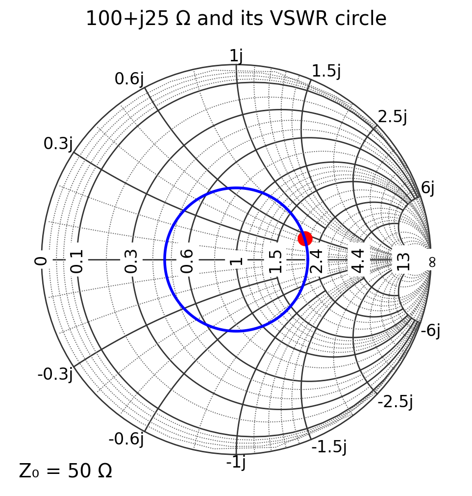
VSWR for a point

Given a complex impedance, VSWR depends on how far that point is from the match in the \(\Gamma\) sense. Below we compute VSWR for a sample impedance and show its circle.

Z0 = 50
Z_load = 100 + 1j * 25

vswr = utils.calc_vswr(Z0, Z_load)

plt.figure(figsize=(6, 6))
ax = plt.subplot(111, projection="smith")

ax.plot(Z_load, "ro", ms=10)
ax.plot_vswr(vswr, "b", label=f"VSWR={vswr:.2f}")

ax.set_title(f"{Z_load.real:.0f}+j{Z_load.imag:.0f} Ω and its VSWR circle")
plt.show()